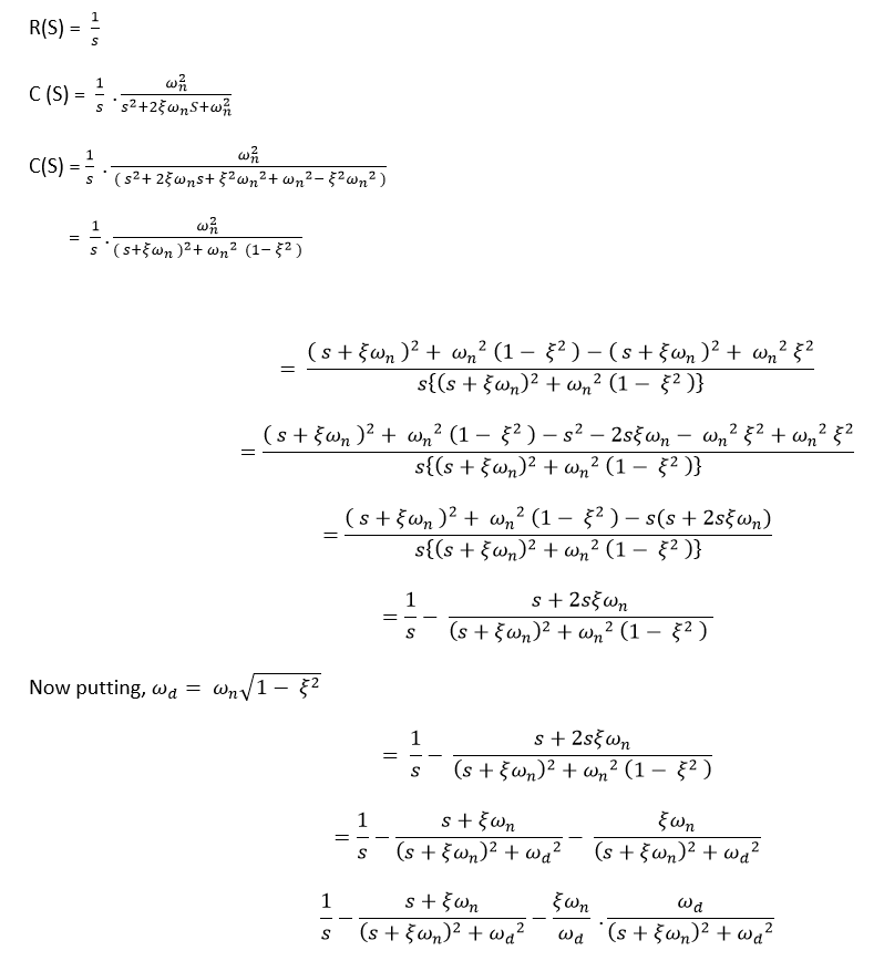
Consider Three Systems Which Have the Following Transfer Functions
The transfer function can thus be viewed as a generalization of the concept of gain. Simple repeated and conjugate poles.
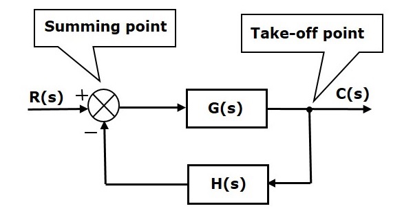
Control Systems Block Diagrams
As the substitution of these values in the denominator leads to provide infinite transfer function.
. Lets calculate the transfer function of the first loop. Transfer Function Analysis For Mechanical Systems For the system shown below do the following. Solving the transfer function Xs Fs 1 5s2 5s 28 1 5 s2 28 5 Rev.
Transform the numbers to the logarithmic domain. The transfer function of the system is bs as and the inverse system has the transfer function as bs. AWriting the equation of motion yields 5s25s28Xs Fs.
Answer 1-8 for the RC circuit below 1. Find the impulse response of the system in time domain. MATLAB Program 3-5 produces four transfer functions.
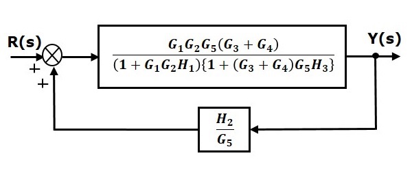
Transfer functions are a frequency-domain representation of linear time-invariant systems. Consider the following transfer functions. The transfer function of a loop is G 1GH We will first simplify the above block diagram into the simple system.
5 The zeros are and the poles are Identifying the poles and zeros of a transfer function aids in understanding the behavior of the system. Additive Property Suppose that an output is influenced by two inputs and that the transfer functions are known. Consider the system defined by This system involves two inputs and two outputs.
X_ 1 x_ 2 2 0 0 3 x 1 x 2 1 1 u 14 y 1 3 x 1 x 2 15 Example 3. Transfer functions of complex systems can be represented in block diagram form. Consider the following transfer function 2s 3 HS - 2 6s 13 a.
X_ 2 6 4 0 1 0 0 0 1 3 2 5 3 7 5x 2 6 4 0 0 10 3 7 5r y h 1 0 0 i x. We can easily find the step input of a system from its transfer function. U1 U2 Ys G11sUsG2sU2s The graphical representation or block diagram is.
Ys Xs cdot Hs. When considering input u we assume that input u2 is zero and vice versa Solution. We now have two distinct poles.
The open-loop transfer function of a feedback control system is - Gs Hs rm frac1s13 The gain margin of the system is - Q4. B Calculate the step response of the system c Use MATLAB to compute the step response numerically. Identify whether the system is an underdamped critically damped or overdamped system.
Fall 2004 Question I Transfer functions of RLC RL and RC Circuits 52 points Circuit A. The open-loop poles are located at s 0 s -3 j4 and s -3 - j4. These are the poles of the above transfer function.
For example consider the transfer function This function has three poles two of which are negative integers and one of which is zero. Obtain the state-space representation of the transfer function system 16 in the controllable canonical form. MATLAB Program 3-5 A O 1 -25 -41.
Addsubtract easy in the log domain to multiplydivide difficult in the linear domain. The tf model object can represent SISO or MIMO transfer functions. TF 1 40s2 1 2 40s2 1 40s 4 Now two blocks are left in cascade.
AFind the transfer function Gs XsFs. G overall s G 1 s G 2 s The overall transfer function for a system composed of elements in series is the product of the transfer functions of the individual series elements. For instance consider a continuous-time SISO dynamic system represented by the transfer function syss NsDs where s jw and Ns and Ds are called the numerator and denominator polynomials respectively.
Find the differential equation representing the system. The poles of a transfer function generally are of three types. The overall transfer function G s of the system is Y s X s and so.
Each part of each problem is worth 3 points and the homework is worth a total of 42 points. Multiplicationdivision of large numbers is difficult. Consider the system presented by the following transfer function ys s2 S s² 2s 3 The A.
Find the transfer function for the above circuit. Find the undamped natural frequency the damped natural frequency and the damping ratio b. Gs s2 3s 3 s2 2s.
YlsUls YsUs YsU2s and Y2sU2s. Let we have a system with transfer function. Notice the symmetry between yand u.
Using the method of partial fractions this transfer function can be written as. Sate space model A state-space model is a discrete. State Space Representation to Transfer Function Find the transfer function Gs YsRs for the following system represented in state space.
The roots of as are called poles of the system. Questions about Transfer Functions These questions should help you with question 3 of quiz 1. To have poles of the transfer function.
Sketch the root loci of the control system shown in Figure 6-40a. A system has a pair of complex conjugate poles p1p2 1 j2 a single real zero z1 4 and a gain factor K 3. Whether the transfer function is proper or improper 2.
Order of the system a b s 3² ss² 10 Gs s1s2s 3 Gs 3D. Extra effort is required but the problem is simplified. 1Transfer functions in series 2Transfer functions in parallel 3Transfer functions in feedback form.
The equivalent block is the product of these two blocks as given below. Use partial fraction expansion d. Given a system with input xt output yt and transfer function Hs Hs fracYsXs the output with zero initial conditions ie the zero state output is simply given by.
S3 s2 91s 67 2. The inverse system is obtained by reversing the roles of input and output. N OS T s T pand T r.
A Determine if the system is critically damped underdamped or overdamped. G1s G2s Ys U1s U2s. 10 02232014 1 of 9.
Consider three systems which have the following transfer functions. Poles of the system 3. 10s 16 32 32 32 4s 16 For each system.
12 12 and Ys Ys Gs Gs Us Us Then the response to changes in both and can be written as. For this we can write the transfer function 13 in the following form. Homework 3 - Solutions Note.
Apply the inverse transform to get back to the original domain. 3 basic arrangements of transfer functions. Hence we get A 1 and B 3.
The transfer function is HsK sz sp1sp2 3 s4 s1j2s1j2 3 s4 s2 2s5 7 and the differential equation is d2y dt2 2 dy dt 5y3 du dt 12u 8. Zeros of the system 4. I HS ii HS -2 8s 16 iüi Hs.
2 points Hjω 2. Four transfer functions are involved. A root locus branch exists on the real.
A control system in which the control action is somehow dependent on the output is known as -.
Time Response Of Second Order Control System Worked Example Electrical4u

The Unit Impulse Response
![]()
Transfer Function Of Control System Electrical4u
![]()
Initial Value Theorem Of Laplace Transform Electrical4u
![]()
Control System Transfer Function Javatpoint
Time Response Of Second Order Control System Worked Example Electrical4u
![]()
Transfer Function Of Control System Electrical4u
![]()
Transfer Function Of Control System Electrical4u

Transfer Function Youtube
Control Systems Block Diagram Reduction
Control System Time Response Of Second Order System Javatpoint
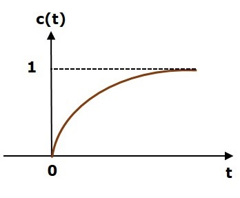
Response Of The First Order System
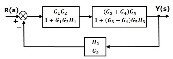
Control Systems Block Diagram Reduction
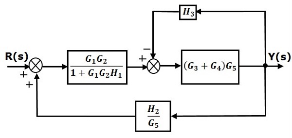
Control Systems Block Diagram Reduction
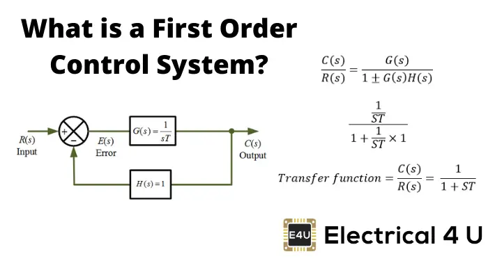
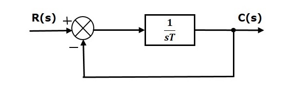
First Order Control System What Is It Rise Settling Time Formula Electrical4u
![]()
Control System Transfer Function Javatpoint
Response Of The First Order System
![]()
Final Value Theorem In Laplace Transform Proof Examples Electrical4u
![]()
Transfer Function Of Control System Electrical4u


Comments
Post a Comment